
Controlling the page layout
✨experimental✨
There are a few ways to control the layout of a page with Jupyter Book. Many of these ideas take inspiration from the Edward Tufte layout CSS guide.
Our plot
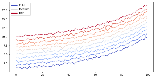
Let's begin with a sample plot. Here's the code we'll use:
# Fixing random state for reproducibility
np.random.seed(19680801)

N = 10
data = [np.logspace(0, 1, 100) + .2 * np.random.randn(100) + ii for ii in range(N)]
data = np.array(data).T
cmap = plt.cm.coolwarm
rcParams['axes.prop_cycle'] = cycler(color=cmap(np.linspace(0, 1, N)))


from matplotlib.lines import Line2D
custom_lines = [Line2D([0], [0], color=cmap(0.), lw=4),
                Line2D([0], [0], color=cmap(.5), lw=4),
                Line2D([0], [0], color=cmap(1.), lw=4)]

fig, ax = plt.subplots(figsize=(10, 5))
lines = ax.plot(data)
ax.legend(custom_lines, ['Cold', 'Medium', 'Hot']);
For example, here's some popout content! It was created by adding the
popout tag to a cell in the notebook. Jupyter Book automatically converts these
cells into helpful side content.
Add a popout cell by adding popout to your cell's tags. Here's what the
cell metadata for a popout cell looks like:
{
    "tags": [
        "popout",
    ]
}
Popouts behave differently depending on the screen size. If the screen is narrow enough, the popout will exist in-line with your content. Make the screen wider and it'll pop out to the right.
Look to the right and play around with your window width to see how this looks!
You can include images in popouts! For example, let's see what the plot above looks like in a popout window.
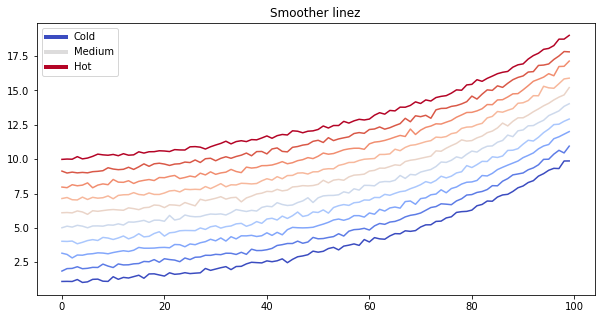
My popout explanation. Since we've put a markdown cell underneath the code above,
we can turn this into a popout as well, and use it as a quick caption to explain
the content above (we have hidden the code for the above plot with a remove_input
tag). However, in the case of this figure, there's not a whole lot to explain :-)
Quotations
There are two types of quotations in Jupyter Book: blockquotes and epigraphs.
Blockquotes are useful for calling out some information provided by another source. They don't break much with the content of the page.
Here's an example of a blockquote. It is triggered by using the "caret" (
>) symbol at the beginning of each line that you'd like to add a blockquote for. If you finish the quote with a-symbol, it will be treated as an "attribution" line and will be right-aligned.
- Jo the Jovyan
Epigraphs are useful for introducing a particular page or idea. They're inspired by Edward Tufte's epigraph CSS. Epigraphs have a bit more emphasis and also differ in style a bit more from your page's content in order to draw attention to them.
Here's an example of an epigraph quote. Note that in this case, the quote itself is a bit larger and italicized. You probably shouldn't make this too long so that they don't stand out too much.
- Jo the Jovyan
To indicate that you'd like an epigraph instead of a blockquote, add the following tag your cell's tag list:
{
    "tags": [
        "epigraph",
    ]
}
Wide-format cells
Sometimes, you'd like to use all of the horizontal space available to you. This allows you to highlight particular ideas, visualizations, etc.
In Jupyter Book, you can specify that a cell (and its outputs) should take up all of the horizonal space (including the sidebar where popouts normally live) using the following cell metadata tag:
{
    "tags": [
        "full_width",
    ]
}
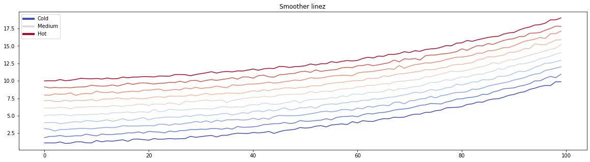
For example, let's take a look at the figure at full-width. We'll tell Matplotlib to make it a bit wider so we can take advantage of the extra space!
# Fixing random state for reproducibility
np.random.seed(19680801)

N = 10
data = [np.logspace(0, 1, 100) + .1*np.random.randn(100) + ii for ii in range(N)]
data = np.array(data).T
cmap = plt.cm.coolwarm
rcParams['axes.prop_cycle'] = cycler(color=cmap(np.linspace(0, 1, N)))


from matplotlib.lines import Line2D
custom_lines = [Line2D([0], [0], color=cmap(0.), lw=4),
                Line2D([0], [0], color=cmap(.5), lw=4),
                Line2D([0], [0], color=cmap(1.), lw=4)]

fig, ax = plt.subplots(figsize=(20, 5))
lines = ax.plot(data)
ax.legend(custom_lines, ['Cold', 'Medium', 'Hot'])
ax.set(title="Smoother linez");
Be careful about mixing popouts and full-width content. Sometimes these can conflict with one another in visual space. You should use them relatively sparingly in order for them to have their full effect of highlighting information.